PCA: Income Data with R

Using tidymodels

1 Introduction

This document demonstrates how to perform Principal Component Analysis (PCA) in R using the tidymodels framework. PCA is a dimensionality reduction technique that transforms a set of possibly correlated variables into a set of linearly uncorrelated variables called principal components. We will use the adult_income_dataset.csv for this demonstration.

2 Load Data

First, we load the necessary libraries and the income dataset.

Code

library(tidyverse)
library(tidymodels)
library(factoextra)

income_data <- read_csv("../data/adult_income_dataset.csv")

# For simplicity, we'll remove rows with any missing values and the 'income' column
income_data_clean <- income_data %>%
  select(-income) %>%
  na.omit() %>%
  sample_n(1000) # Randomly sample 10,000 rows

# Preprocessing using recipes
income_recipe <- recipe(~ ., data = income_data_clean) %>%
  step_rm(all_nominal_predictors()) %>% # One-hot encode all nominal (categorical) predictors
  step_normalize(all_numeric_predictors()) %>% # Normalize all numerical predictors
  prep(training = income_data_clean)

income_data_processed <- bake(income_recipe, new_data = income_data_clean)

# Remove any columns that might have resulted in all zeros after one-hot encoding if they were constant
income_data_processed <- income_data_processed[, colSums(income_data_processed) != 0]

Code

glimpse(income_data_processed)

Rows: 1,000
Columns: 6
$ age              <dbl> 1.30127420, 0.49702562, -0.89213102, -1.25769855, 0.4…
$ fnlwgt           <dbl> 0.14594412, 0.02091497, -0.72304477, 0.47604431, 1.46…
$ `education-num`  <dbl> 0.00320406, 0.00320406, 1.60523414, 0.40371158, 1.204…
$ `capital-gain`   <dbl> -0.1346700, -0.1346700, -0.1346700, -0.1346700, 1.020…
$ `capital-loss`   <dbl> -0.2088594, -0.2088594, -0.2088594, -0.2088594, -0.20…
$ `hours-per-week` <dbl> -0.08372406, -0.08372406, 0.31918287, -0.08372406, 0.…

3 Principal Component Analysis

We will perform PCA on the preprocessed income data.

Code

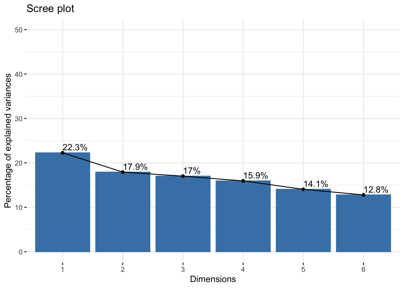
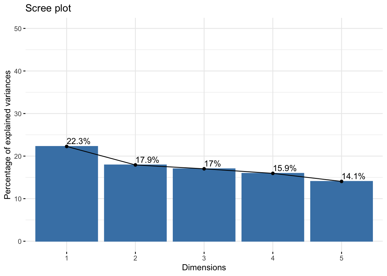
# Perform PCA
res.pca <- prcomp(income_data_processed, scale = FALSE) # Data is already scaled

# Visualize eigenvalues (scree plot)
fviz_eig(res.pca, addlabels = TRUE, ylim = c(0, 50))

4 PCA Results Visualization

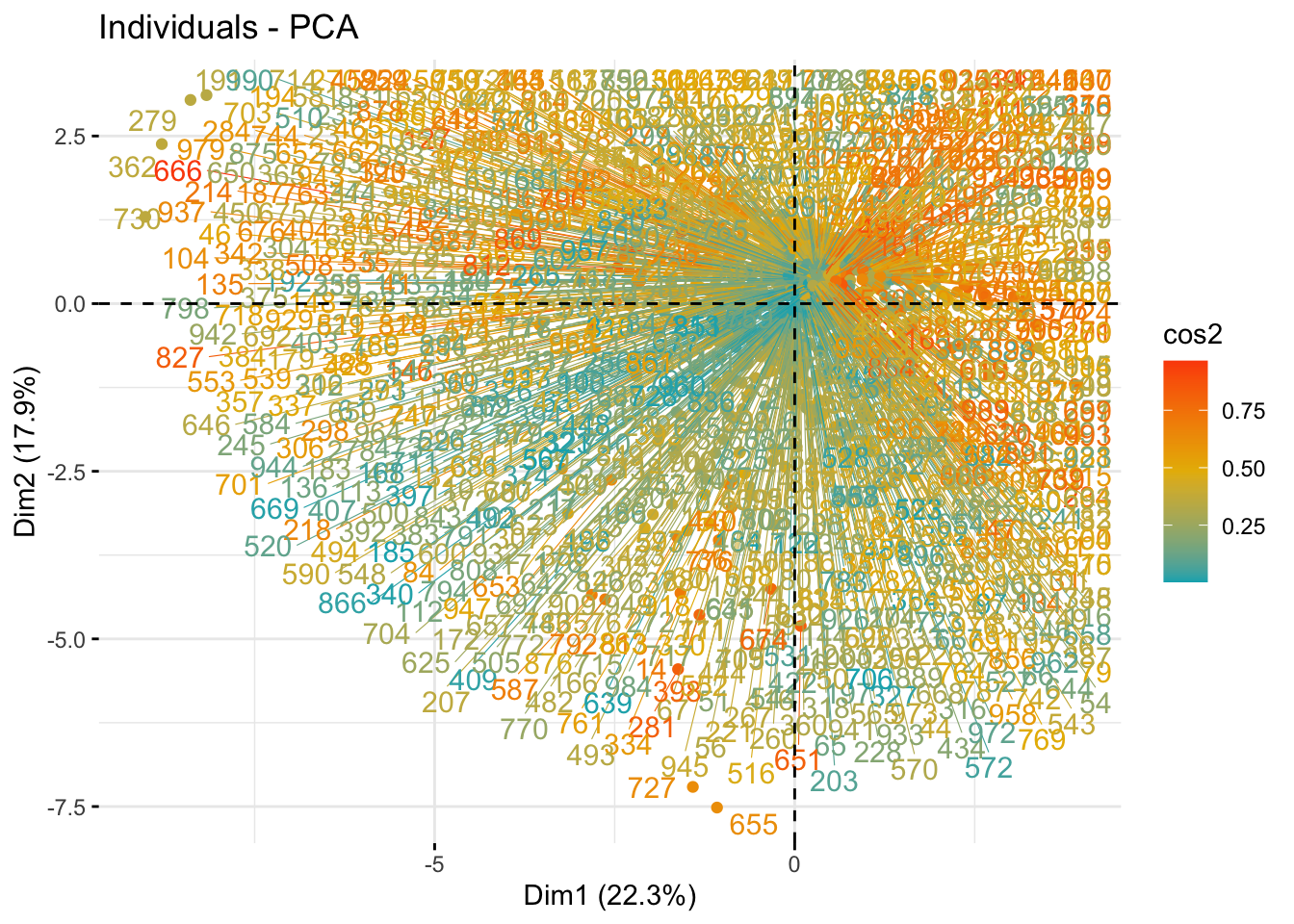
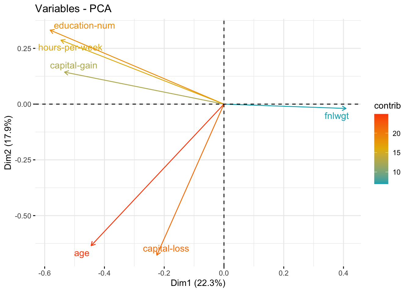
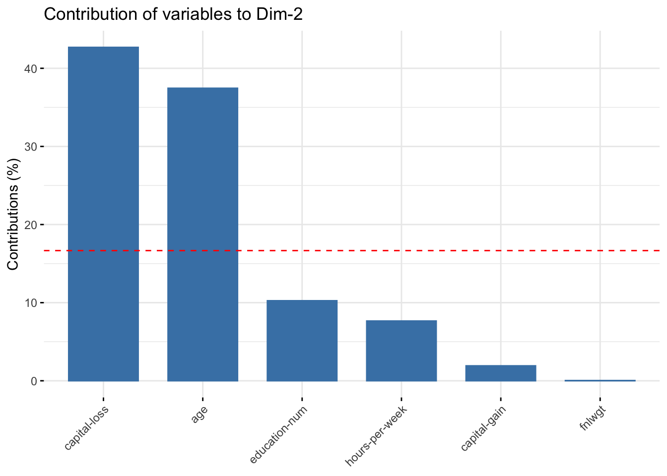
We can visualize the results of PCA, including the contribution of variables to the principal components and the individuals’ positions.

Code

# Plot of individuals on the first two principal components
fviz_pca_ind(res.pca,
             col.ind = "cos2", # Color by the quality of representation
             gradient.cols = c("#00AFBB", "#E7B800", "#FC4E07"),
             repel = TRUE,     # Avoid text overlapping
             ggtheme = theme_minimal()
             )

Code

# Plot of variables
fviz_pca_var(res.pca,
             col.var = "contrib", # Color by contributions to the PC
             gradient.cols = c("#00AFBB", "#E7B800", "#FC4E07"),
             repel = TRUE,     # Avoid text overlapping
             ggtheme = theme_minimal()
             )

Code

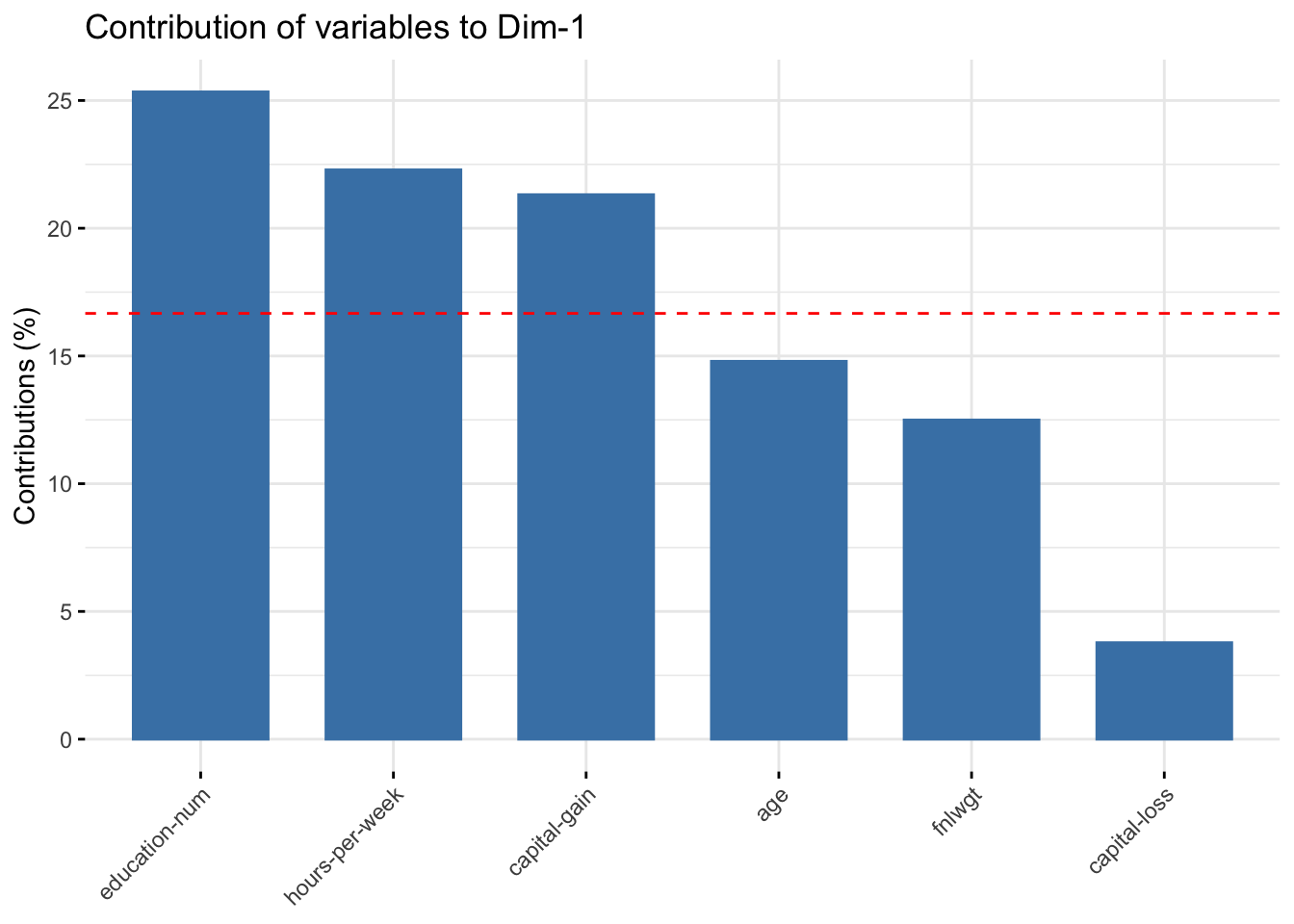
# Contributions of variables to PC1
fviz_contrib(res.pca, choice = "var", axes = 1, top = 10)

Code

# Contributions of variables to PC2
fviz_contrib(res.pca, choice = "var", axes = 2, top = 10)

Code

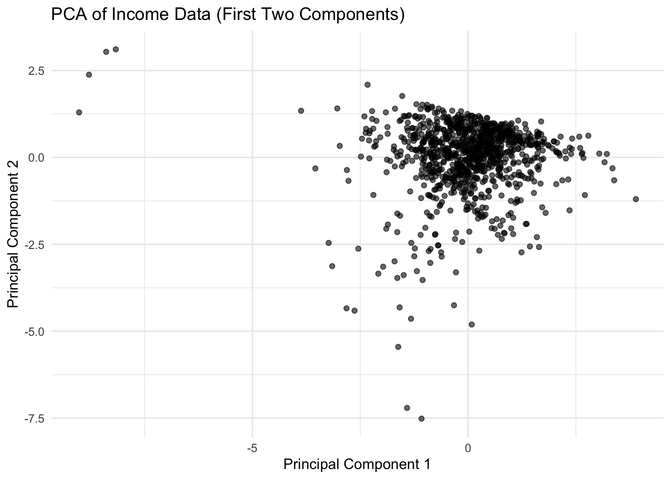
# 2D scatter plot of individuals on the first two principal components (similar to Python)
# Extract the principal components
pca_coords <- as.data.frame(res.pca$x)

# Plot using ggplot2
ggplot(pca_coords, aes(x = PC1, y = PC2)) +
  geom_point(alpha = 0.6) +
  labs(title = "PCA of Income Data (First Two Components)",
       x = "Principal Component 1",
       y = "Principal Component 2") +
  theme_minimal()

5 Conclusion

This document provided an overview of Principal Component Analysis in R using tidymodels. We demonstrated how to perform PCA on the income dataset and visualize the results.If your data is mostly categorical, PCA is often not the best choice. Use these instead.

6 Keeping Top 5 Components

We can select and work with a reduced number of principal components, for example, the top 5 components that explain a significant portion of the variance.

Code

# Get the principal components (coordinates of the individuals)
head(res.pca$x[, 1:5])

             PC1        PC2        PC3         PC4         PC5
[1,] -0.30820157 -0.7034257  0.4603546  0.21892956  0.20877998
[2,] -0.04308345 -0.2088990  0.2588782  0.02618587  0.05519673
[3,] -0.76839229  1.2796291 -0.4834717 -0.74272659 -1.02196672
[4,]  0.59105267  0.9846954 -0.6859196  0.11686084 -0.41102262
[5,] -0.86178201  0.4203588 -0.6879925  1.72778722 -0.15791388
[6,] -0.06130784 -0.9194863  2.0712145 -0.42712528  0.03847342

Code

# Get the loadings (eigenvectors)
head(res.pca$rotation[, 1:5])

                      PC1        PC2        PC3         PC4         PC5
age            -0.3845978 -0.6119846  0.3307280  0.13142952  0.16486731
fnlwgt          0.3534702 -0.0187077 -0.5159685  0.69617116  0.16787246
education-num  -0.5033651  0.3202052 -0.3236615  0.01110994 -0.63251341
capital-gain   -0.4616662  0.1384811  0.2893874  0.66679350  0.01273139
capital-loss   -0.1943652 -0.6533350 -0.5481655 -0.08689269 -0.16162932
hours-per-week -0.4720735  0.2767127 -0.3679786 -0.21397349  0.71991546

Code

# Visualize the variance explained by the first 5 components
fviz_eig(res.pca, addlabels = TRUE, ylim = c(0, 50), ncp = 5)

--- title: "PCA: Income Data with R" subtitle: "Using tidymodels" execute: warning: false error: false format: html: toc: true toc-location: right code-fold: show code-tools: true number-sections: true code-block-bg: true code-block-border-left: "#31BAE9" --- ## Introduction This document demonstrates how to perform Principal Component Analysis (PCA) in R using the `tidymodels` framework. PCA is a dimensionality reduction technique that transforms a set of possibly correlated variables into a set of linearly uncorrelated variables called principal components. We will use the `adult_income_dataset.csv` for this demonstration. ## Load Data First, we load the necessary libraries and the income dataset. ```{r} #| label: load-data #| echo: true library(tidyverse) library(tidymodels) library(factoextra) income_data <- read_csv("../data/adult_income_dataset.csv") # For simplicity, we'll remove rows with any missing values and the 'income' column income_data_clean <- income_data %>% select(-income) %>% na.omit() %>% sample_n(1000) # Randomly sample 10,000 rows # Preprocessing using recipes income_recipe <- recipe(~ ., data = income_data_clean) %>% step_rm(all_nominal_predictors()) %>% # One-hot encode all nominal (categorical) predictors step_normalize(all_numeric_predictors()) %>% # Normalize all numerical predictors prep(training = income_data_clean) income_data_processed <- bake(income_recipe, new_data = income_data_clean) # Remove any columns that might have resulted in all zeros after one-hot encoding if they were constant income_data_processed <- income_data_processed[, colSums(income_data_processed) != 0] ``` ```{r} glimpse(income_data_processed) ``` ## Principal Component Analysis We will perform PCA on the preprocessed income data. ```{r} #| label: pca #| echo: true # Perform PCA res.pca <- prcomp(income_data_processed, scale = FALSE) # Data is already scaled # Visualize eigenvalues (scree plot) fviz_eig(res.pca, addlabels = TRUE, ylim = c(0, 50)) ``` ## PCA Results Visualization We can visualize the results of PCA, including the contribution of variables to the principal components and the individuals' positions. ```{r} #| label: pca-viz #| echo: true # Plot of individuals on the first two principal components fviz_pca_ind(res.pca, col.ind = "cos2", # Color by the quality of representation gradient.cols = c("#00AFBB", "#E7B800", "#FC4E07"), repel = TRUE, # Avoid text overlapping ggtheme = theme_minimal() ) # Plot of variables fviz_pca_var(res.pca, col.var = "contrib", # Color by contributions to the PC gradient.cols = c("#00AFBB", "#E7B800", "#FC4E07"), repel = TRUE, # Avoid text overlapping ggtheme = theme_minimal() ) # Contributions of variables to PC1 fviz_contrib(res.pca, choice = "var", axes = 1, top = 10) # Contributions of variables to PC2 fviz_contrib(res.pca, choice = "var", axes = 2, top = 10) # 2D scatter plot of individuals on the first two principal components (similar to Python) # Extract the principal components pca_coords <- as.data.frame(res.pca$x) # Plot using ggplot2 ggplot(pca_coords, aes(x = PC1, y = PC2)) + geom_point(alpha = 0.6) + labs(title = "PCA of Income Data (First Two Components)", x = "Principal Component 1", y = "Principal Component 2") + theme_minimal() ``` ## Conclusion This document provided an overview of Principal Component Analysis in R using `tidymodels`. We demonstrated how to perform PCA on the income dataset and visualize the results.If your data is mostly categorical, PCA is often not the best choice. Use these instead. ## Keeping Top 5 Components We can select and work with a reduced number of principal components, for example, the top 5 components that explain a significant portion of the variance. ```{r} #| label: top-5-components-r #| echo: true # Get the principal components (coordinates of the individuals) head(res.pca$x[, 1:5]) # Get the loadings (eigenvectors) head(res.pca$rotation[, 1:5]) # Visualize the variance explained by the first 5 components fviz_eig(res.pca, addlabels = TRUE, ylim = c(0, 50), ncp = 5) ```